Various data are organized, processed, and interpreted every second for different applications to improve human life. 

From the annual income of residents of a particular province and the recent census to the monthly sales of various companies and your quarterly academic grades, all these things involve data and information that must be collected and organized to extract valuable insights. 

This is what statistics are for. Statistics is collecting, organizing, interpreting, and presenting data. To kick off our statistics review, we will discuss the measures of central tendency: the mean, median, and mode.

Click below to go to the main reviewers:

Ultimate Civil Service Exam Reviewer

Ultimate NMAT Reviewer

Ultimate PMA Entrance Exam Reviewer

Ultimate NAPOLCOM Exam Reviewer

Ultimate UPCAT Reviewer

Ultimate LET Reviewer

An Overview of Statistics

Before we delve into the measures of central tendency, you must have a refresher about the branch of mathematics called statistics.

We have already defined that statistics refers to the science of collecting, organizing, interpreting, and presenting data. And when we say “data,” we refer to any information we can collect and organize. For instance, your age, current school, annual family income, and even your favorite color can be data for statistical ventures.

There are two branches of statistics: descriptive statistics and inferential statistics.

Descriptive statistics is the one we are more familiar with. It is the creation of graphs, tables, and charts and summarizing data to provide valuable insights and interpretations. On the other hand, inferential statistics is about creating point or interval estimation for testing a specific hypothesis regarding a population from a given sample. It is the more complex side of statistics.

In this review, we will focus only on descriptive statistics, specifically, the measures of central tendency. 

Measures of Central Tendency

Suppose you are a researcher who wants to identify the current performance of a particular group of 500 students in their algebra class. To determine the students’ performance, you have asked their teachers for their test scores from their latest algebra exam. 

After providing you with the scores of the 500 students in their algebra exam, you are overwhelmed by the tremendous amount of data. The scores vary, with some students having excellent scores while some have considerably mediocre scores. Are there any ways for you to interpret the data you have in hand? 

This is where measures of central tendency come into the picture. They allow you to describe a given data set using only one value representing the “middle” or the center of the data distribution.

So, going back to your data with 500 students’ algebra scores, you can interpret this staggering amount of data using one single value in the middle of the distribution of these scores. 

What are the measures of central tendency?

The most familiar to us is the mean or average. However, there’s also what we call “median” and “mode,” which provide helpful interpretations like the mean.

Let us discuss these measures of central tendency one by one.

1. Mean

The “mean” or “average” is the most familiar (and most commonly used) measure of the central tendency of a particular group of data. 

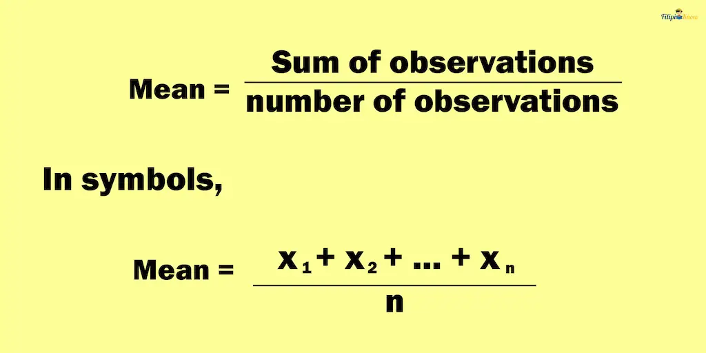
The mean is the sum of the given observations (the term used for the elements of a given data) divided by the total number of observations. 

Here’s a simple example:

Suppose you have the following scores from your four quizzes in your algebra class: 92, 85, 80, and 91. What is your mean score?

It’s pretty basic – add your scores: 92 + 85 + 80 + 91 = 348

Then, divide the sum (which is 348) by the number of observations or scores you have (you have four observations): 348/4 = 87

Thus, your mean score is 87.

Well, your mean score in your algebra class is not bad so far!

Sample Problem 1: Below are the total sales garnered by Mr.Santos’ hardware shop for this week. Mr. Santos is considering whether he should continue his hardware shop business. He has decided that if his mean sales for this week are less than ₱5,000, he will stop his hardware shop business and think of a new one.

Based on the data below, should Mr. Santos continue his hardware shop business?

Day	Total Sales
Monday	₱3,200
Tuesday	₱5,000
Wednesday	₱6,300
Thursday	₱3,500
Friday	₱6,000

Solution:

Adding the daily sales of Mr. Santos:

3,200 + 5,000 + 6,300 + 3,500 + 6,000 = 24,000

Since we have five observations, we divide 24,000 by 5:

24,000/5 = 4,800

Thus, the mean sales of Mr. Santos is ₱4,800, which is less than ₱5,000. Based on these findings, Mr. Santos should stop his hardware shop business and consider a new one.

Sample Problem 2: Luke’s mean score in his five statistics quizzes is 92. What is the sum of Luke’s scores on his five statistics quizzes?

Solution: We know that the mean is the result when we divide the sum of the observations by the total number of observations or:

 mean = sum of observations ÷ number of observations

 mean of Luke’s scores = sum of Luke’s scores ÷ number of scores

Let x be the sum of Luke’s scores in his five statistics quizzes. Since Luke’s mean score is 92 and there are five quiz scores, then:

mean of Luke’s scores = sum of Luke’s scores ÷ number of scores ➡ 92 = x⁄5

We have the linear equation: 92 = x⁄5

To solve for x in 92 = x⁄5, we multiply both sides of the equation by 5:

5(92) =5(x⁄5)

460 = x

x = 460

Therefore, the value of x, the sum of  Luke’s scores in his five statistics quizzes, is 460. 

From this example, you might have discovered that the sum of the values of the given observations is just the product of the mean of those observations and the total number of observations.

Sample Problem 3: The current average score for Fred from his five previous basketball games is 21. Suppose that in their team’s sixth game, Fred contributed 17 points. What will be Fred’s average score for the six previous games? 

Solution: We need to determine first what Fred’s total score is from his six previous games. Fred’s total score from his last six games is the sum of the following:

Fred’s total score in his five previous games + Fred’s score in his sixth game

Fred’s score in his sixth game is 17. While we still don’t know his total score in his previous games, Fred’s average score from his five previous basketball games is 21.

Fred’s total score in his five previous games is just the product of his average score and the total number of observations or scores (5). Thus, Fred’s total score in his five previous games is 21 x 5 = 105.

This means that Fred’s total score for his six previous games is: 105 + 17 = 122

We divide 122 by 6 to find Fred’s average score for his six previous games: 122/6 = 20.33

Thus, the answer for this example is 20.33.

Although the mean is an effective measure of central tendency, it also has its share of weaknesses. One of its flaws is its vulnerability to being influenced by “outliers.” 

Outliers are values that are either too high or too low compared to the other values in a given set of data.

For example, suppose your scores in your five previous 50-item mathematics exams are 45, 48, 47, 44, and 10. For whatever reason, you obtained a really low score in your last mathematics exam. Noticeably, 10 is very low compared to the other scores, all greater than 40. Thus, we can consider 10 as an outlier. 

Let us compute the mean: [45 + 48 + 47 + 44 + 10] ÷ 5 = 38.8

As you can see, because of that outlier value of 10, the mean is now considered not a good representative of your scores since most are greater than 40. Notice how that single outlier value changed your mean score drastically (this also means that you must be consistent with your test scores!). 

Properties of the Mean

Here are some other things you must remember about mean or average:

1. The mean of a given set of data does not need to be an element of the given set of data

For example, the mean of the set of numbers {1, 2, 3, and 8} is 3.5. Notice that 3.5 is not an element of the given set of data. 

2. The sum of the deviations from the mean is always 0

The deviation is the difference when you subtract the mean from an element of a given data set. If you add these deviations, the result will always be 0.

For example, the mean of the set of numbers {1, 2, 3, and 8} is 3.5. Suppose we subtract 3.5 from each element of the data set:

1 – 3.5 = -2.5

2 – 3.5 = -1.5

3 – 3.5 = -0.5

8 – 3.5 = 4.5

The deviations are -2.5, -1.5, -0.5, and 4.5. Adding them:

-2.5 + (-1.5) + (-0.5) + 4.5 = 0

3. If you add (or subtract) each observation by the same certain real number, the mean will be increased (or decreased) by that real number

The mean of the set of numbers {1, 2, 3, and 8} is 3.5. Suppose that we increase each observation by 3:

1 + 3 = 4

2 + 3 = 5

3 + 3 = 6

8 + 3 = 11

So, the new observations are {4, 5, 6, and 11}. If we take their mean, we have:

[4 + 5 + 6 + 11] ÷ 4 = 6.5

The mean is 6.5. Notice that 6.5 will be the value we obtain if we add 3 to the mean of the original observations (i.e., 3.5 + 3 = 6.5).

2. Median

To get the median, arrange the given values in an ascending or descending order, then take the value in the middle. That middle value is the median.

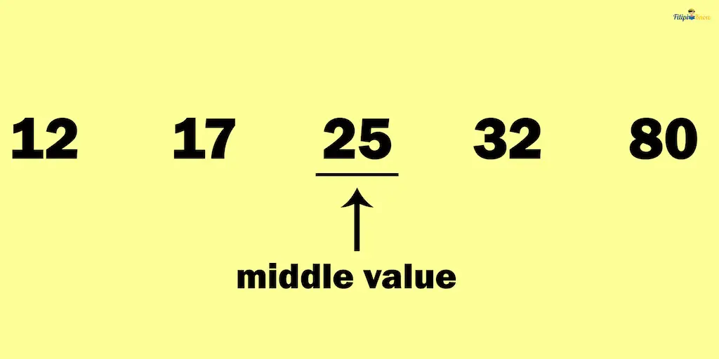
Suppose you have the following values:  32, 12, 25, 17, and 80. If you want to determine their median, the first thing you have to do is to arrange the values in an ascending (or descending) order:

12, 17, 25, 32, 80

After we have arranged the given values, we take the middle value. The middle value is 25. Therefore, the median of the given values is 25.

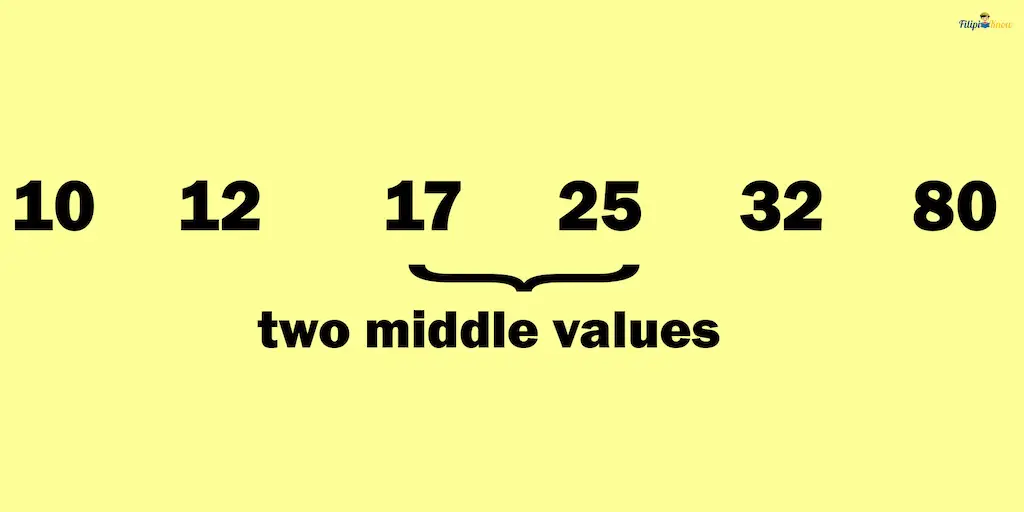
However, if the number of observations is even, you must make additional computations to obtain the median. For instance, suppose we want to identify the median of these given observations: 32, 12, 25, 17, 80, and 10.

If we arrange the values in ascending order, we have

10, 12, 17, 25, 32, and 80

Notice that we will not obtain a single number if we try to take the middle value. Instead, we will get numbers precisely 17 and 25. This is because we have six observations, and six is an even number.

To identify the median of a data set with an even number of observations, we take these two “middle” values and obtain their average or mean. So, in our example above, the two “middle” values are 17 and 25. Obtaining their average:

[17 + 25] ÷ 2

42 ÷ 2

21

The average of 17 and 25 is 21. Therefore, the median of the given set of observations should be 21.

We summarize below the steps on how to find the median of a set of numbers:

How To Determine the Median of a Set of Numbers (or Observations)

1. If the Number of Observations Is Odd

Step 1: Arrange the given numbers in an ascending or descending order.

Step 2: Identify the middle value or observation; the middle observation is the median.

2. If the Number of Observations Is Even

Step 1: Arrange the given numbers in an ascending or descending order.

Step 2: Identify the two middle values or observations.

Step 3: Get the mean or average of the two middle values.

Step 4: The resulting mean or average is the median.

Sample Problem 1: Given below are the heights of eleven Grade 10 high school students of a particular national high school:

172 cm, 168 cm, 169 cm, 169 cm, 171 cm, 168 cm, 169 cm, 173 cm, 170 cm, 168 cm, 170 cm

Determine the median height.

Solution: There are eleven observations. Therefore, we will use the steps in determining the median of a set of numbers if the number of observations is odd:

Step 1: Arrange the given numbers in an ascending or descending order.

We arrange the set of observations in ascending order (you can also arrange it in descending order and still end up with the same answer).

168 cm, 168 cm, 168 cm, 169 cm, 169 cm, 169 cm, 170 cm, 170 cm, 171 cm, 172 cm, 173 cm

Step 2: Identify the middle value or observation; the middle observation is the median.

Based on the list, the middle value is the 6th observation:

168 cm, 168 cm, 168 cm, 169 cm, 169 cm, 169 cm, 170 cm, 170 cm, 171 cm, 172 cm, 173 cm

Thus, the middle value is 169 cm.

This means that the median height of the eleven Grade 10 students is 169 cm.

Sample Problem 2: Below are the ages of eighteen known physicists in a particular city. 

32

45

42

31

33

33

48

38

39

42

42

41

46

38

38

39

37

39

Identify the median age of the physicists.

Solution: The number of observations we have is 18, which is an even number. Therefore, we will use the steps to determine the median if the number of observations is even. 

Step 1: Arrange the given numbers in an ascending or descending order.

31

32

33

33

37

38

38

38

39

39

39

41

42

42

42

45

46

48

After arranging the given values, we can proceed to the second step.

Step 2: Identify the two middle values or observations

The middle values are the 9th and the 10th observations:

31

32

33

33

37

38

38

38

39

39

39

41

42

42

42

45

46

48

As we can see, the 9th and the 10th observations are both 39.

Step 3: Get the mean or average of the two middle values.

(39 + 39)/2 = 78/2 = 39

Step 4: The resulting mean or average is the median.

The resulting mean we calculated in the previous step is 39. Then, the median age of the physicists is 39.

Some Properties of the Median

1. The median divides the given set of observations or the distribution into two equal parts

Consider the given set of observations {3, 4, 5, 6, 7}. The median of this set of observations is 5. On the left of 5, there are two observations which are 3 and 4. On the other hand, on the right of 5, there are also two observations which are 6 and 7. Indeed, the median value divided the observations into two equal parts.

2. The median is less affected by outliers

Unlike the mean, the median is not affected by outliers. 

Consider the set of observations {3, 4, 5, 6, 7}; the median of this set of data is 5.

Suppose that we replace one of the observations with a meager value. Let’s say we replace 3 with 0.003. We will have the following observations: {0.003, 4, 5, 6, 7}. Note that even with the presence of the outlier, the median is still 5. 

Now, suppose that we replace 6 with an outlier value of 120. We have 

{3, 4, 5, 7, 120} 

Notice that the median value is still 5.

3. Mode

If you have a given set of data, there are possible values that are repeated or occur frequently. Mode refers to the most commonly occurring value or observation in a set of observations. 

Simply put, the mode is the observation mostly repeated in a given set of observations.

Consider the following observations: 1, 2, 2, 3, 4, 5, 6, 7

Notice that the value of 2 is repeated twice in the above set, while the rest appeared only once. Hence, 2 is the most commonly occurring value. Therefore, the mode of the set of observations above is 2.

The mode of a given set of observations can be more than one number. For example, consider the observations: 1, 2, 2, 3, 3, 4, 5, 6, 7. Notice that observations 2 and 3 are the most commonly occurring values. Hence, the modes of this set of observations are 2 and 3.

If there are two modes in a set of observations, we call it bimodal. On the other hand, if there are more than two modes, we call it multimodal.

Sample Problem 1: Determine the modal age of a group of mathematicians in a specific city using the data below.

32, 55, 34, 36, 39, 39, 39, 40, 35, 30

Solution: Among the given ages of the mathematicians, the most commonly repeated age is 39. Hence, the modal age is 39. 

Sample Problem 2: A group of researchers surveyed what subject some college students love the most. Determine the mode of the survey results given the data below.

Subject	Frequency
Algebra and Trigonometry	59
Introductory Economics	57
Philippine History	60
English for Academic Writing	58
Physical Education	60
Earth Science	64

Solution: We can interpret the given data above as follows:

Fifty-nine students said they loved Algebra and Trigonometry, 57 said Introductory Economics, 60 students loved Philippine History, and so on.

Based on the given data above, we can state that the subject most commonly repeated as a response by the students in the survey is Earth Science, with 64 students who said that they love it. Therefore, the mode of the survey is Earth Science.

Note: It is incorrect to state that the mode of the data above is 64 since it is the number of times that “Earth Science” was repeated as the most loved subject and not a response to the survey itself. Hence, the correct mode of this data is “Earth Science.”

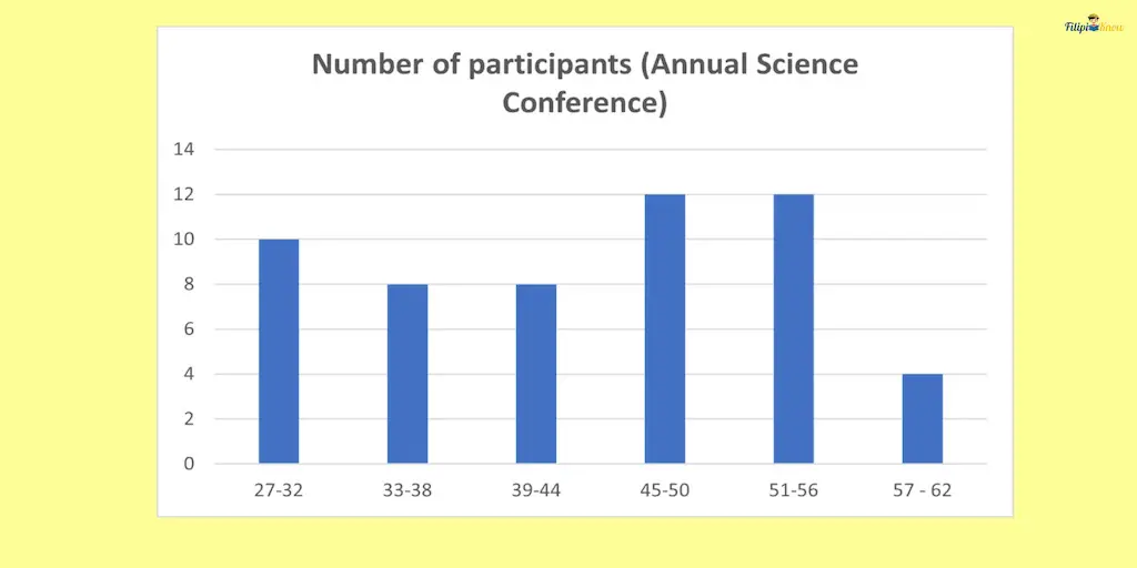
Sample Problem 3: Look at the graph below featuring the ages of the participants of an annual science conference. Determine the modal age group.

Solution: Based on the graph, the age group with the highest frequency or number of participants are 45-50 and 51-56. Therefore, we have a bimodal measure. The modal age groups are 45-50 yrs. old and 51-56 yrs. old.

Next topic: Probability

Previous topic: Unit Circle

Return to the main article: The Ultimate Basic Math Reviewer

Download Printable Summary/Review Notes

Download Printable Flashcards

Test Yourself!

1. Practice Questions [Free PDF Download]

2. Answer Key [Free PDF Download]

3. Math Mock Exam + Answer Key